Planewave simulation - Implementation of more accurate multislice algorithms for low energy TEM

Updated: 16 Mar 2026

This notebook takes you through a simple planewave simulation for the same crystal used in the thesis and creates a RGB overlay to compare the differences. Feel free to play around with the simulation parameters like the electron energy.

import abtem
import ase
import matplotlib.pyplot as plt
import numpy as np

Creating the crystal¶

STO_crystal = ase.Atoms(
    "SrTiO3",
    scaled_positions=[
        (0.0, 0.0, 0.0),

        (0.5, 0.5, 0.5),

        (0.5, 0.0, 0.5),
        (0.5, 0.5, 0.0),
        (0.0, 0.5, 0.5),
    ],
    cell=[3.91270131, 3.91270131, 3.91270131, 90, 90, 90],
    pbc=True
)
STO_orthorhombic = abtem.orthogonalize_cell(STO_crystal)

fig,ax = plt.subplots()
abtem.show_atoms(STO_orthorhombic,plane='yz',scale=0.5,tight_limits=True,show_periodic=True,ax=ax)

(<Figure size 640x480 with 1 Axes>, <Axes: xlabel='y [Å]', ylabel='z [Å]'>)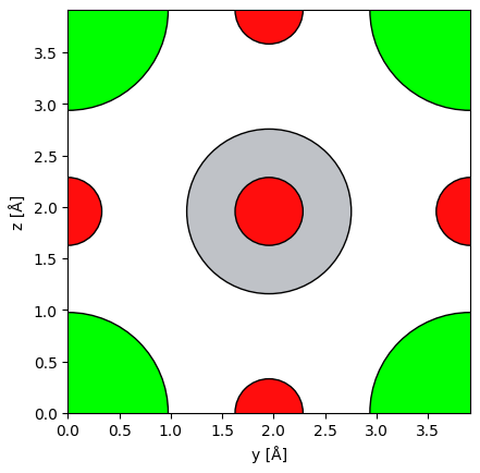

Creating the crystal potential¶

sampling = 0.1 #Angstrom
slice_thickness = 0.5 #Angstrom
thickness = 48 #unit cells 
sample_size = (1,1,thickness)
energy = 20e3 #eV

unit_cell_potential = abtem.Potential(
            STO_orthorhombic,
            sampling=sampling,
            parametrization="lobato",
            slice_thickness=slice_thickness,
            projection="finite",
        )

potential = abtem.CrystalPotential(
    unit_cell_potential,
    repetitions=sample_size,
)

Creating the planewave¶

planewave = abtem.PlaneWave(energy=energy).match_grid(potential)

Running the simulation¶

from abtem.multislice import RealSpaceMultislice 

detector = abtem.PixelatedDetector(max_angle=None)

CMS = RealSpaceMultislice()
PCMS = RealSpaceMultislice(
    order = 3,
)
FCMS = RealSpaceMultislice(
    order = 3,
    expansion_scope='full'
)

CMS¶

exitwave_cms = planewave.multislice(
    potential=potential,
    detectors=detector,
    algorithm = CMS,
    pbar=True,
    lazy=False
    )

exitwave_pcms = planewave.multislice(
    potential=potential,
    detectors=detector,
    algorithm = PCMS,
    pbar=True,
    lazy=False
    )

exitwave_fcms = planewave.multislice(
    potential=potential,
    detectors=detector,
    algorithm = FCMS,
    pbar=True,
    lazy=False
    )

all_exitwaves = abtem.stack(
    (
        exitwave_cms.block_direct(),
        exitwave_pcms.block_direct(),
        exitwave_fcms.block_direct()
    ),
    (
        'CMS',
        'PCMS',
        'FCMS'
    )
)

all_exitwaves.show(
    explode = True,
    cbar=True,
    cmap='magma',
    figsize=(16, 9),
    vmin=0,
    common_color_scale=True,
    power=0.5
)

<abtem.visualize.visualizations.Visualization at 0x142ad47d0>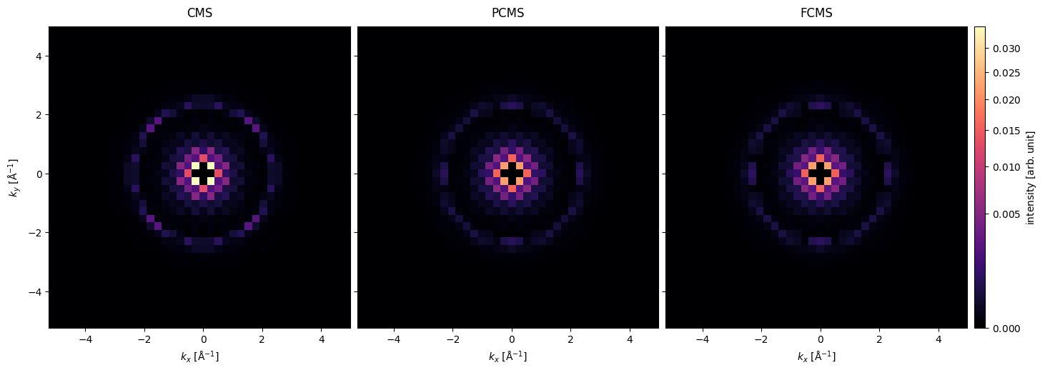

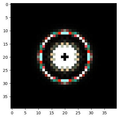
RGB overlay¶

threshold = 0.95

cms_array = exitwave_cms.block_direct().array
R_quantile = np.quantile(cms_array, threshold)
cms_array = np.clip(cms_array, 0, R_quantile)
R = cms_array / cms_array.max()

pcms_array = exitwave_pcms.block_direct().array
G_quantile = np.quantile(pcms_array, threshold)
pcms_array = np.clip(pcms_array, 0, G_quantile)
G = pcms_array / pcms_array.max()

fcms_array = exitwave_fcms.block_direct().array
B_quantile = np.quantile(fcms_array, threshold)
fcms_array = np.clip(fcms_array, 0, B_quantile)
B = fcms_array / fcms_array.max()

rgb_image = np.stack([R, G, B], axis=-1)
plt.imshow(rgb_image, vmin=0)