(PA)CBED simulation - Implementation of more accurate multislice algorithms for low energy TEM

Updated: 16 Mar 2026

This notebook takes you through a simple CBED simulation for the same crystal used in the thesis and creates a RGB overlay to compare the differences. Feel free to play around with the simulation parameters like the electron energy. This notebook also does a PACBED scan and compares the different models for that as well.

import abtem
import ase
import matplotlib.pyplot as plt
import numpy as np

STO_crystal = ase.Atoms(
    "SrTiO3",
    scaled_positions=[
        (0.0, 0.0, 0.0),

        (0.5, 0.5, 0.5),

        (0.5, 0.0, 0.5),
        (0.5, 0.5, 0.0),
        (0.0, 0.5, 0.5),
    ],
    cell=[3.91270131, 3.91270131, 3.91270131, 90, 90, 90],
    pbc=True
)
STO_orthorhombic = abtem.orthogonalize_cell(STO_crystal)

abtem.show_atoms(STO_orthorhombic,plane='yz',scale=0.5,tight_limits=True,show_periodic=True)

(<Figure size 640x480 with 1 Axes>, <Axes: xlabel='y [Å]', ylabel='z [Å]'>)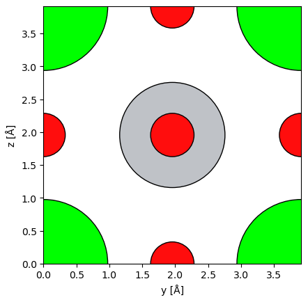

sampling = 0.1 #Angstrom
slice_thickness = 0.5 #Angstrom
thickness = 48 #unit cells 
sample_size = (12,12,thickness)
energy = 20e3 #eV
semiangle=20

unit_cell_potential = abtem.Potential(
            STO_orthorhombic,
            sampling=sampling,
            parametrization="lobato",
            slice_thickness=slice_thickness,
            projection="finite",
            # device='gpu'
        )

potential = abtem.CrystalPotential(
    unit_cell_potential,
    repetitions=sample_size,
)

probe = abtem.Probe(
    energy=energy,
    semiangle_cutoff=semiangle,
    # device='gpu'
).match_grid(potential)

probe.show()

<abtem.visualize.visualizations.Visualization at 0x7614f8340a10>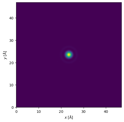

from abtem.multislice import RealSpaceMultislice 

detector = abtem.PixelatedDetector(max_angle=None)

CMS = RealSpaceMultislice()
PCMS = RealSpaceMultislice(
    order = 3,
)
FCMS = RealSpaceMultislice(
    order = 3,
    expansion_scope='full'
)

exitwave_cms = probe.multislice(potential=potential,detectors=detector, algorithm = CMS,pbar=True,lazy=False)

exitwave_pcms = probe.multislice(potential=potential,detectors=detector, algorithm = PCMS,pbar=True,lazy=False)

exitwave_fcms = probe.multislice(potential=potential,detectors=detector, algorithm = FCMS,pbar=True,lazy=False)

all_exitwaves = abtem.stack(
    (
        exitwave_cms,
        exitwave_pcms,
        exitwave_fcms
    ),
    (
        'CMS',
        'PCMS',
        'FCMS'
    )
)

all_exitwaves.show(
    explode = True,
    cbar=True,
    cmap='magma',
    figsize=(16, 9),
    vmin=0,
    common_color_scale=True,
    power=0.5
)

<abtem.visualize.visualizations.Visualization at 0x7614b8cffb90>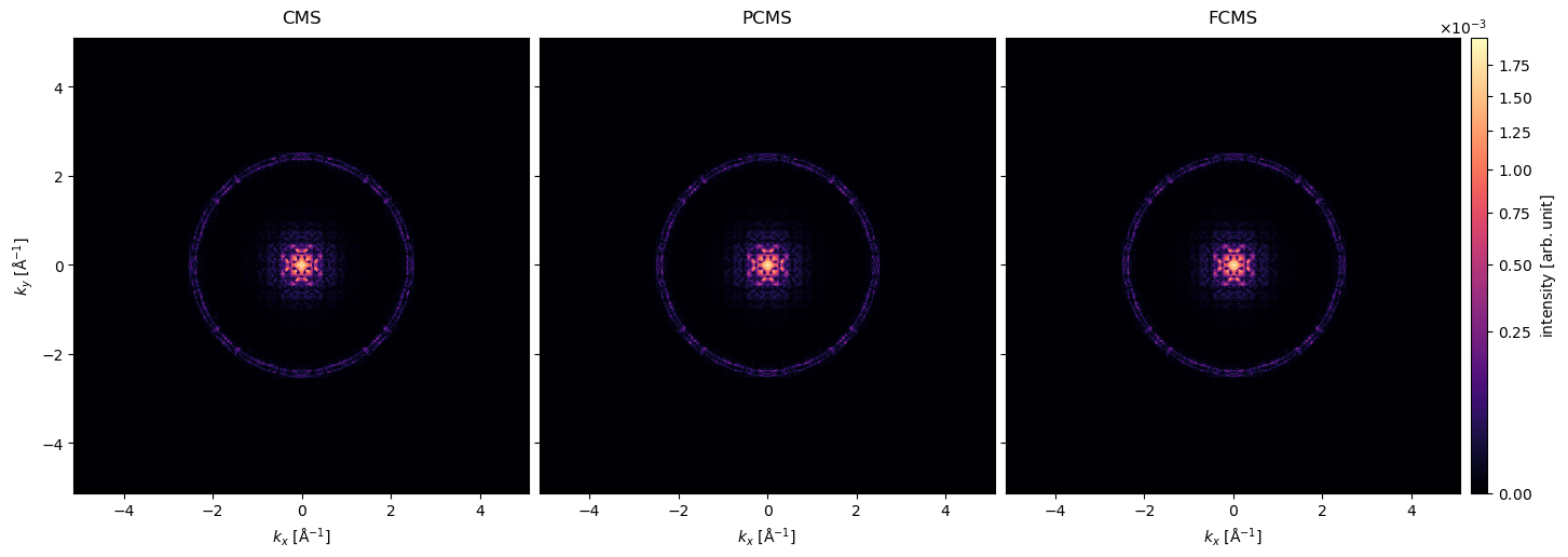

threshold = 0.98

cms_array = exitwave_cms.array
R_quantile = np.quantile(cms_array, threshold)
cms_array = np.clip(cms_array, 0, R_quantile)
R = cms_array / cms_array.max()

pcms_array = exitwave_pcms.array
G_quantile = np.quantile(pcms_array, threshold)
pcms_array = np.clip(pcms_array, 0, G_quantile)
G = pcms_array / pcms_array.max()

fcms_array = exitwave_fcms.array
B_quantile = np.quantile(fcms_array, threshold)
fcms_array = np.clip(fcms_array, 0, B_quantile)
B = fcms_array / fcms_array.max()

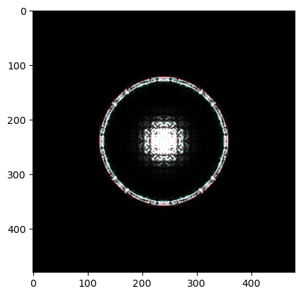
rgb_image = np.stack([R, G, B], axis=-1)
plt.imshow(rgb_image, vmin=0)

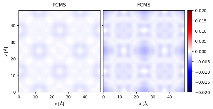
PACBED¶

Here we perform a PACBED scan for a higher electron energy and plot the relative difference between the PCMS/FCMS and the CMS as explained in Section. STEM.

haadf = abtem.AnnularDetector(inner=25, outer=None)

probe = abtem.Probe(energy=200e3, semiangle_cutoff=semiangle, device='gpu').match_grid(potential)

grid_scan = abtem.GridScan(
    start=[0, 0],
    end=(STO_orthorhombic.cell[0,0]*1, STO_orthorhombic.cell[1,1]*1),
    sampling=probe.aperture.nyquist_sampling,
    potential=potential,
)

fig, ax = abtem.show_atoms(STO_orthorhombic*(12,12,1))
grid_scan.add_to_plot(ax)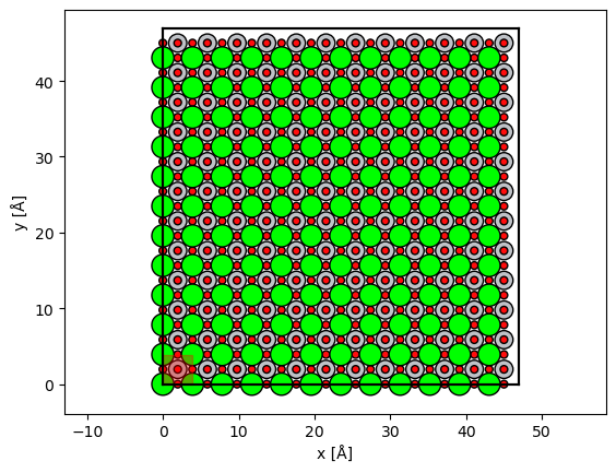

measurements_cms = probe.scan(potential, scan=grid_scan, detectors=haadf, lazy=False, algorithm=CMS, pbar=True)

measurements_pcms = probe.scan(potential, scan=grid_scan, detectors=haadf, lazy=False, algorithm=PCMS, pbar=True)

measurements_fcms = probe.scan(potential, scan=grid_scan, detectors=haadf, lazy=False, algorithm=FCMS, pbar=True)

interpolation_value = 0.05

all_exitwaves = abtem.stack(
    (
        measurements_cms.tile((2,2)).interpolate(sampling=interpolation_value),
        measurements_pcms.tile((2,2)).interpolate(sampling=interpolation_value),
        measurements_fcms.tile((2,2)).interpolate(sampling=interpolation_value)
    ),
    (
        'CMS',
        'PCMS',
        'FCMS'
    )
)

all_exitwaves.show(
    explode = True,
    cbar=True,
    cmap='inferno',
    figsize=(14, 8),
    common_color_scale=True,
)

<abtem.visualize.visualizations.Visualization at 0x7614b033f4d0>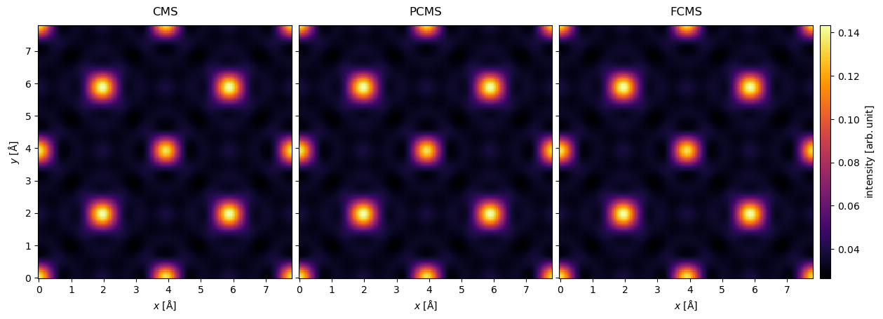

from abtem.measurements import Images

diff_rel_pcms = (measurements_pcms.tile((2,2)).interpolate(sampling=interpolation_value).array - measurements_cms.tile((2,2)).interpolate(sampling=interpolation_value).array) / (1e-6 + measurements_cms.tile((2,2)).interpolate(sampling=interpolation_value).array)
diff_rel_fcms = (measurements_fcms.tile((2,2)).interpolate(sampling=interpolation_value).array - measurements_cms.tile((2,2)).interpolate(sampling=interpolation_value).array) / (1e-6 + measurements_cms.tile((2,2)).interpolate(sampling=interpolation_value).array)

diff_rel_pcms_img = Images(array = diff_rel_pcms, sampling=probe.aperture.nyquist_sampling)
diff_rel_fcms_img = Images(array = diff_rel_fcms, sampling=probe.aperture.nyquist_sampling)

all_measurements = abtem.stack(
    (
        diff_rel_pcms_img,
        diff_rel_fcms_img
    ),
    (
        'PCMS',
        'FCMS'
    )
)

all_measurements.show(
    cmap='seismic', 
    vmin=-0.02, 
    vmax=0.02, 
    explode=True, 
    figsize=(8, 5),
    common_color_scale=True,
    cbar=True
)

<abtem.visualize.visualizations.Visualization at 0x7614991ee250>