Transmission electron microscopy
Transmission electron microscopy (TEM) is a wave-based microscopy technique, similar to light microscopy, where the illumination by photons is replaced by electrons. These electrons, like photons, have a certain wavelength derived from the de Broglie wavelength, which states that the wavelength of a particle is inversely proportional to its momentum.
Therefore, the wavelength of electrons can be orders of magnitude smaller than their photonic counterpart. When the object of interest approaches the scale of the wavelength with which it is imaged, diffraction causes the individual points to blend together. Thus with a smaller wavelength, a higher resolution can be achieved when imaging with electrons.
A TEM consists of a source of free moving electrons followed by a series of electromagnetic lenses which focus the beam on the specimen Williams & Carter (2009). These electrons are accelerated using an electrostatic potential known as the accelerating voltage. The beam passes through an aperture which controls the maximum angle in the beam as well as the intensity of the electron current reaching the detector.
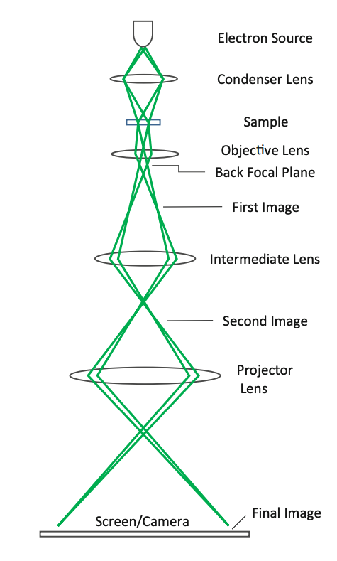
Figure 1:Diagram of a basic TEM Zuo & Spence (2017)
This beam of electrons then passes through the sample where due to its potential the electrons undergo scattering. This scattering thus provides information of the electrostatic potential of the sample which is ultimately the quantity of interest. The scattered electrons, after leaving the sample, are either magnified to form an image or, for all instances in this thesis, detected by a detector in the far field. This separates the electrons based on their wavevector generating a diffraction pattern. The interpretation of this diffraction pattern is where the simulation of this process is very useful since it is then possible to simulate what caused the patterns with various optical parameters.
Ewald spheres
The sample of interest is often a crystal with atoms arranged in a pattern which is periodic in real space. To understand the scattering effects of the electrons, it is useful to view the lattice in reciprocal space. Because the realspace crystal lattice is periodic, when we calculate its potential in realspace, it can be represented by a Fourier series. The different wavevectors making up the Fourier series can be plotted in reciprocal space. Assuming that the scattering happens elastically, the energy is preserved and thus also the wavelength. This means that for any scattered electron, its wavelength must be the same as that of the incident electron. Since the electron can scatter to any direction but must keep its wavelength, in reciprocal space this translates to a sphere with radius whose surface represents all possible scattering directions. This sphere is called the Ewald sphere. In order for a electron to be detected after the sample, the contributions from all atoms must interfere constructively. This means that the contributions from different atoms must have a phase difference of any integer multiple of . By way of Braggs law, only scattering directions with a change in wavevector equal to one of the reciprocal lattice points can meet this requirement, assuming the origin is the unscattered beam. Combining the two criteria: only lattice points in reciprocal space that land on the Ewald sphere are valid scattering direction.
Conventional multislice
The conventional multislice (CMS) algorithm is a method to simulate the scattering effects of the electron beam by the sample. To see how the multislice method works we begin by stating the problem the multislice algorithm tries to solve. The incoming electron beam can be described by its wavefunction: , whose absolute square tells you the probability of finding an electron when measured. When this wavefunction enters the sample, it obeys the so-called time-independent, relativistically corrected Schrödinger equation.
Because the CMS assumes a high velocity along the optical axis, we can write the wavefunction as:
Here we have also separated the from the full position vector . Substituting this into Eq.(2) and dropping the second derivative compared to because it is assumed to be a slow moving envelope, as demonstrated by Ming & Chen (2013), yields:
The CMS begins by dividing the sample potential into N different slices, where each slice is defined by Chen & Van Dyck (1997):
This new potential per slice can be substituted into Eq.(2) and solving this differential equation gives the solution
Using this formula, the wavefunction after each slice can be calculated with the wavefunction coming into that slice. Thus starting with the beam wavefunction and recursively calculating the next wavefunction for each sample slice, we end up with the final electron wavefunction, known as the exitwave.
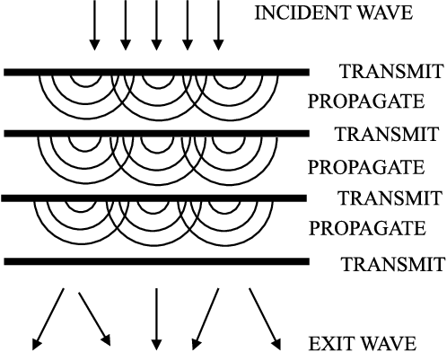
Figure 2:Diagram showing the working of the multislice algorithm Muller et al. (2006)
Numerically, the multislice algorithm can be calculated both in realspace and using a Fourier transform. The latter is the more common approach, since using the fast Fourier transform (FFT) will result in a much faster calculation. If the slice thickness is sufficiently small, Eq.(6) can be rewritten as
The first operator in the exponent is called the Fresnel propagator, while the second is the transmission operator. If we now apply the transmission operator in realspace by multiplying it with the incident wave function, we are left with the transmitted wave. Then the Fourier transform is taken of this transmitted wave and multiplied by the fourier transform of the Fresnel propagator which turns into a simple multiplication.
After that, the inverse Fourier transform is taken to obtain the final wave.
Python implementation
To implement Eq.(6) numerically we start with a discretized illumination wavefunction which is a 2D complex array as well as a 3D potential array. The potential array is already a potential for each slice calculated using Eq.(5). This is handled by the abTEM Madsen & Susi (2021) library with a Waves object and Potential object respectively which handles the array and the metadata like energy and wavelength and also provided a range of functions like detection with detectors and easily scanning a range of positions. Because in Eq.(6) the 2D laplacian is an operator acting on the wavefunction is in the exponent, we need to use the Taylor expansion of the exponent.
To get the power of the multislice operator, we simply apply it times. By using this method it is possible for the series to diverge Zekendorf (2024) depending on slice thickness and sampling size. The code for the conventional multislice operator can be found in Code. 1
Then we can use the exponential series to calculate the exponent of the conventional operator applied to the incident wavefunction Code. 2.
- Williams, D. B., & Carter, C. B. (2009). Transmission Electron Microscopy: A Textbook for Materials Science. Springer US. 10.1007/978-0-387-76501-3
- Zuo, J. M., & Spence, J. C. H. (2017). Advanced Transmission Electron Microscopy: Imaging and Diffraction in Nanoscience. Springer. 10.1007/978-1-4939-6607-3
- Ming, W. Q., & Chen, J. H. (2013). Validities of three multislice algorithms for quantitative low-energy transmission electron microscopy. Ultramicroscopy, 134, 135–143. 10.1016/j.ultramic.2013.04.013
- Chen, J., & Van Dyck, D. (1997). Accurate multislice theory for elastic electron scattering in transmission electron microscopy. Ultramicroscopy, 70(1–2), 29–44. 10.1016/S0304-3991(97)00057-7
- Muller, D. A., Kirkland, E. J., Thomas, M. G., Grazul, J. L., Fitting, L., & Weyland, M. (2006). Room design for high-performance electron microscopy. Ultramicroscopy, 106(11–12), 1033–1040.
- Madsen, J., & Susi, T. (2021). abTEM: Transmission Electron Microscopy from First Principles. Open Research Europe, 1(24), 13015. 10.12688/openreseurope.13015.1
- Zekendorf, R. (2024). Comparing Real-Space and Conventional Multislice in abTEM [Bachelor’s Thesis]. University of Vienna.