Fully Corrected MS - Implementation of more accurate multislice algorithms for low energy TEM

Updated: 16 Mar 2026

Theoretical Framework¶

Improved Multislice¶

Starting from Eq.~\ref{time-independent relativistically corrected Schrödinger equation}, one can come to the following version of the multislice equation, as demonstrated by~\citet{Ming2013}

\varphi_j(\mathbf{R}) = \exp \left[ 2\pi i \varepsilon K_0 \left[ \sqrt{1 + \frac{\Delta}{(2\pi K_0)^2} + \frac{\sigma}{\pi K_0} U_j(\mathbf{R})} - 1 \right] \right] \varphi_{j-1}(\mathbf{R})

(1)

Again we solve the inconvenience of the operator inside the square root by taylor expanding it which results in the following solution to the fully corrected multislice.

\varphi_j(\mathbf{R}) = \exp \left[i \varepsilon \left\{\left[ \frac{\Delta}{4\pi K_0} + \sigma U_j(\mathbf{R}) \right] - \frac{1}{4\pi K_0} \left[ \frac{\Delta}{4\pi K_0} + \sigma U_j(\mathbf{R}) \right]^2 + \frac{1}{8\pi^2 K_0^2} \left[ \frac{\Delta}{4\pi K_0} + \sigma U_j(\mathbf{R}) \right]^3 - \dots \right\} \right] \varphi_{j-1}(\mathbf{R})

(2)

This formula is a power series of the part inside the exponent of the original CMS and for that reason we can calculate the nth power by applying the the same function used to calculate the inside of the exponent $n$ times.

Backscattering¶

Besides the improvement in accuracy achieved by Eq.(1) we can also simulate the backscattering effect where the electrons have a small chance of backscattering of the sample. We define a wave vector operator Chen et al. (2025)

\widehat{\boldsymbol{k}_j}(\boldsymbol{R}) = \pm K_0 \sqrt{1 + \frac{1}{(2\pi K_0)^2}\Delta + \frac{\sigma}{\pi K_0}U_j(\boldsymbol{R})}

(3)

Using this operator we define a backscattering operator

\widehat{\boldsymbol{B}}_{j+1, \quad j} = \frac{\widehat{\boldsymbol{k}}_{j+1} - \widehat{\boldsymbol{k}}_j}{2\widehat{\boldsymbol{k}}_{j+1}} \approx \frac{\sigma}{4\pi K_0}(U_j - U_{j-1})

(4)

With

\widehat{\boldsymbol{k}}(\boldsymbol{R}, j\varepsilon) = K_0 \left\{ 1 + \frac{1}{2\pi K_0} \left[ \frac{\Delta}{4\pi K_0} + \sigma U(\boldsymbol{R}, j\varepsilon) \right] - \frac{1}{8(\pi K_0)^2} \left[ \frac{\Delta}{4\pi K_0} + \sigma U(\boldsymbol{R}, j\varepsilon) \right]^2 + \dots \right\}

(5)

And

\frac{1}{\widehat{\boldsymbol{k}}(\boldsymbol{R}, j\varepsilon)} = \frac{1}{K_0} \left\{ 1 - \frac{1}{2\pi K_0} \left[ \frac{\Delta}{4\pi K_0} + \sigma U(\boldsymbol{R}, j\varepsilon) \right] + \frac{3}{8(\pi K_0)^2} \left[ \frac{\Delta}{4\pi K_0} + \sigma U(\boldsymbol{R}, j\varepsilon) \right]^2 + \dots \right\}

(6)

Applying this operator to the wavefunction for each slice gives the backscattered wave. In general, the amplitude of this backscattered wave is much smaller than the forward scattered wave. This is dependent on the atomic mass of the atoms inside the sample. By looking at the approximation of (4) we can also see a dependence on the wavelength and thus the energy of the electron ( $\sigma/K_0 \propto \lambda^2$ ). We can further improve the forward scattering accuracy of the FCMS by subtracting the backscattered wave from the forward scattered wave.

If we additionally store the backscattered part of the wave at each slice, we can reconstruct the total backscattered wave that would be detected by an upstream detector (i.e. in reflection, without disrupting the incident beam). The total backscattered wave can be reconstructed from the final exitwave Chen & Van Dyck (1997)

\varphi_{backscattered}(\mathbf{R}) = - \sum_{m=1}^{n} \left( \prod_{j=m}^{1} \mathrm{e}^{2\pi \mathrm{i} \hat{k}_j \varepsilon} \right) \left( \widehat{\boldsymbol{B}}_{m+1, m} \mathrm{e}^{2\pi \mathrm{i} \hat{k}_m \varepsilon} \right) \varphi_{N}(\mathbf{R})

(7)

Because the backscattered waves are complex valued, this formula assumes perfect coherence allowing the backscattered waves to interfere with each other. In reality however, this is often not the case and instead the waves are incoherent or partially coherent.

Python Implementation¶

Improved Multislice¶

As described earlier, we can calculate the powers of the conventional multislice step inside the FCMS taylor series by applying the CMS step multiple times. Summing these powers until a chosen order $n$ with the correct prefactor gives us Eq.(2). After which we again use the exponential series to calculate its exponent Code. 4.

Because Eq.(5) and Eq.(6) also use the fully corrected multislice power series we can reuse it, except for the prefactor in Eq.~\ref{khat_operator_reciprocal_taylor_expansion} being slightly different. For this reason, we introduce the ability to override the prefactor.

Backscattering¶

To calculate the total backscattered wave, we need to calculate and store the backscattered wave from each slice which would make up the total wave and multislice each part through the rest of the sample. Calculating the backscattered wave at each slice is done by Code. 5 For storing the backscattered wave at each slice, abTEM provides a functionality we exploit called exit planes which allows the specification of indices where the wavefunction at that slice index is stored in an array. This is very useful to see the forming of the exit wave inside the sample. But, by overriding these exit planes with our backscattered wave at each slice, we can easily calculate the total backscattered wavefunction without heavy modifications to the existing codebase.

Because we store a backscattered wave at each slice and not the operator and since the multislice operator is linear, we can use Eq.(7) in a more efficient way. Starting at the last slice ( $j=N$ ), we take the part of the wave that backscattered at that slice and apply the multislice operator once to take it to slice $N-1$ . There we add the backscattered wave coming from that slice and apply the multislice operator again on this new total wave. This process is repeated for the entire specimen until we reach the entrance surface Code. 6. In the case of fully incoherent waves, the individual backscattered waves from each slice should be summed by their intensities. For that reason this method does not work since we sum as we go through the sample. This is identical to using Eq. (7). Finally, we compute the farfield intensities of this total wave, as it would reach a detector.

Results¶

The same sample and parameters were used as in Propagator Corrected MS. Therefore, the results are presented the same way as that chapter. Also like in Propagator Corrected MS the order of the FCMS operator goes up to the third power.

24 unit cells z thickness

48 unit cells z thickness

Diffraction patterns for SrTiO_3 illuminated by planewave for different energies with 24 unitcells thickness in z axis and power=0.25 — Figure 1:Diffraction patterns for SrTiO $_3$ illuminated by planewave for different energies with 24 unitcells thickness in z axis and power=0.25

24 unit cells z thickness

48 unit cells z thickness

Comparison of the conventional multislice (CMS) and the propagator corrected multislice (FCMS) for SrTiO_3 with 24 unitcells thickness in z axis — Figure 3:Comparison of the conventional multislice (CMS) and the propagator corrected multislice (FCMS) for SrTiO $_3$ with 24 unitcells thickness in z axis

Now we present the total coherent backscattered wavefunction for the same sample of SrTiO3 with 24 unit cells thickness. Note this appears qualitatively different from electron backscattered diffraction (EBSD) patterns, which are incoherent and usually modelled by leveraging the principle of reciprocity Winkelmann (2009).

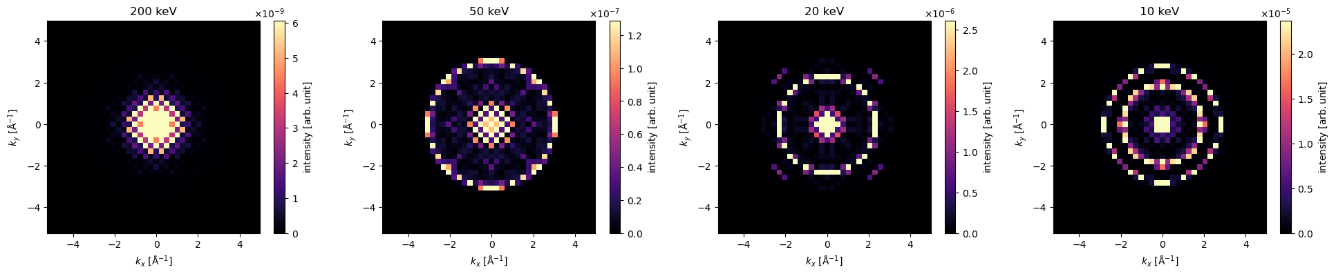
Reconstructed backscattered wave for SrTiO_3 with 24 unitcells thickness in z axis — Figure 5:Reconstructed backscattered wave for SrTiO $_3$ with 24 unitcells thickness in z axis

References¶

Chen, G. S., He, Y. T., Ming, W. Q., Wu, C. L., Van Dyck, D., & Chen, J. H. (2025). Fast STEM image simulation in low-energy transmission electron microscopy by the accurate Chen-van-Dyck multislice method. Micron, 190, 103778. https://doi.org/10.1016/j.micron.2024.103778
Chen, J., & Van Dyck, D. (1997). Accurate multislice theory for elastic electron scattering in transmission electron microscopy. Ultramicroscopy, 70(1–2), 29–44. 10.1016/S0304-3991(97)00057-7
Winkelmann, A. (2009). Dynamical Simulation of Electron Backscatter Diffraction Patterns. In Electron Backscatter Diffraction in Materials Science (pp. 21–33). Springer US. 10.1007/978-0-387-88136-2_2