Planewave Diffraction Comparison
At first glance, the PCMS and FCMS seem to create the same changes compared to the CMS in realspace. There are clear differences in the higher scattering angles between both methods with conventional multislice. To show the differences and similarities between the 3 methods we employ a channel merging approach, where we assign a RGB color to each and plot the composition of all colors. This will result in a greyscale pixel if they agree and otherwise, the pixel will be a different color. We do this for the same sample as in previous chapters with 2 different sample thicknesses.
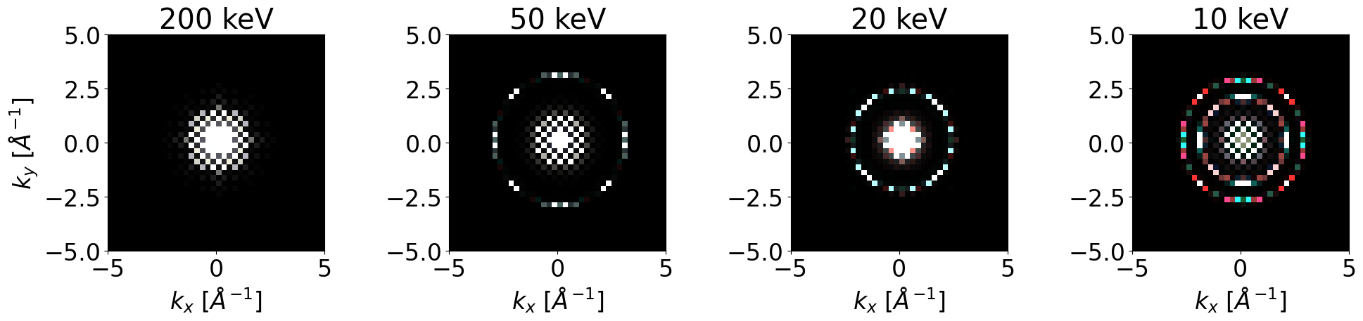
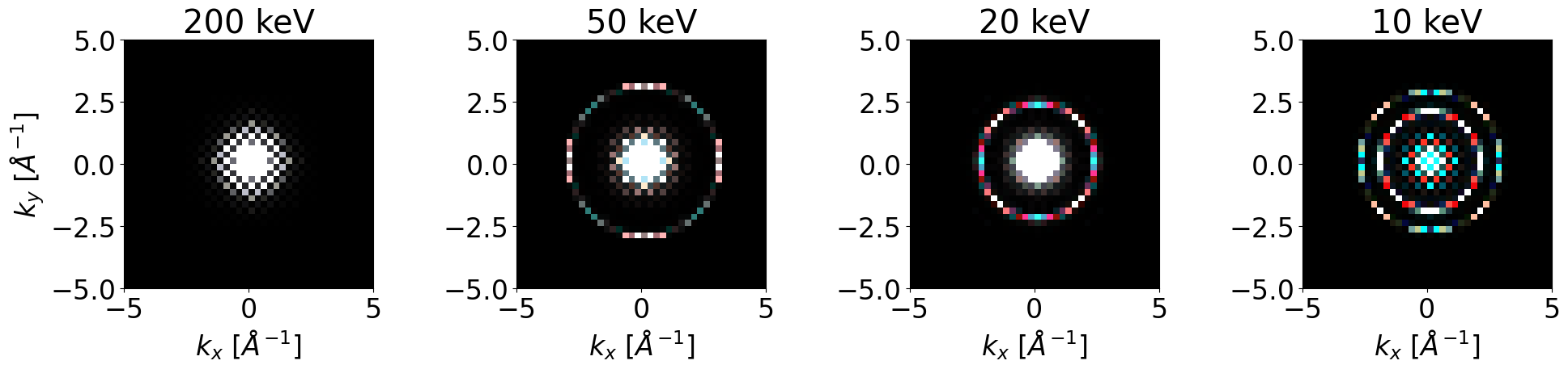
We see that, as the voltage lowers, the CMS and the other 2 methods diverge. Still, at 10 keV, the PCMS and FCMS still mostly agree since we only see red and cyan (green and blue combined in equal proportion). To show the difference between them we can go to an even lower voltage, namely 5 kV.
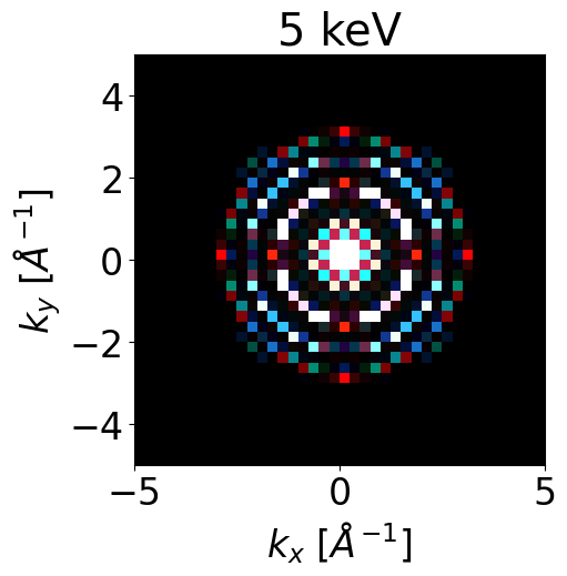

Here we can see clear separation of all 3 colors. From these plots we can observe that the 3 methods differ in terms of high angle scattering.
Converged Probe Comparison
Single scan position
Thus far we have only used planewave illumination. Although this is great for demonstrating the method, it is not possible to create pure planewave illumination in a real TEM. Therefore, we will now perform the same simulation but with a converged probe.
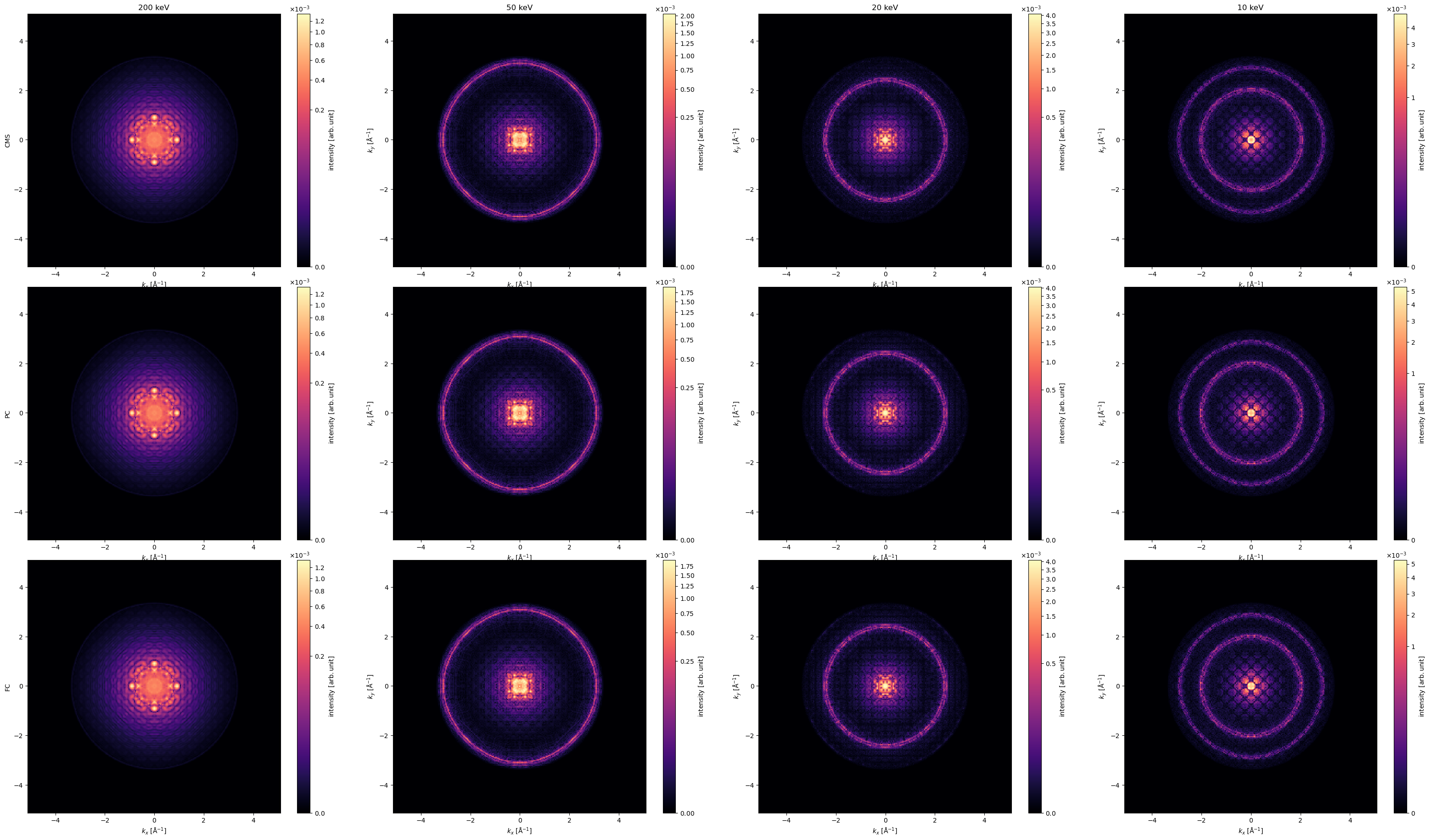
Figure 5:CBED scans for a sample of 8x8x24 unitcells of SrTiO3 for different methods at various energies
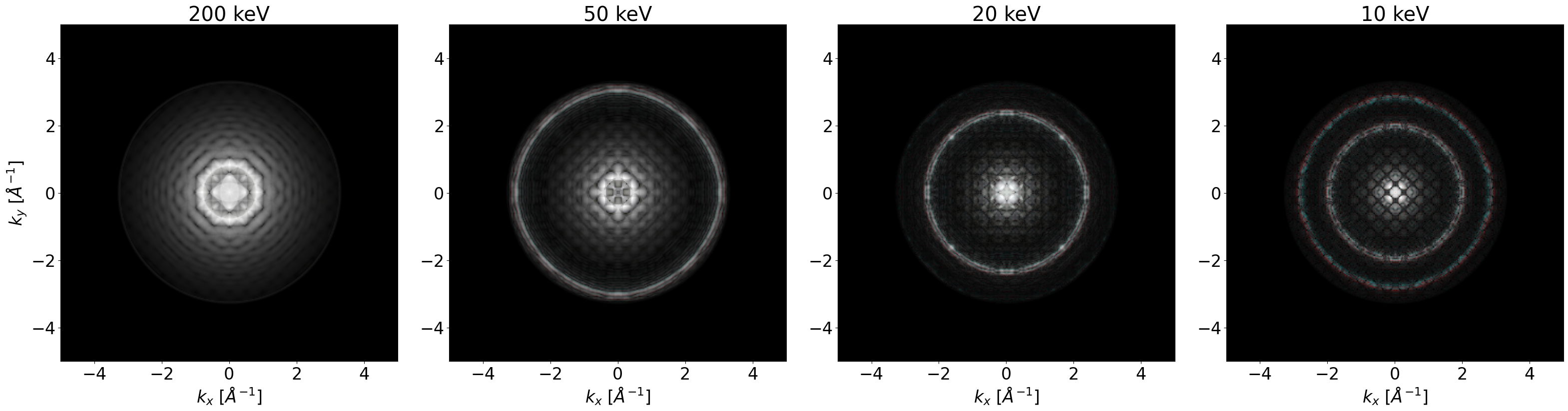
Figure 6:RGB comparison between R = CMS (RS), G = PCMS, B = FCMS for sample thickness 24c for Figure 5
Although less clear than for the planewaves, we again observe a slight separation of red and cyan at 20 keV, which gets more clear at 10 keV.
STEM
Unlike the planewave simulation, the CBED simulation is dependent on its position above the sample. To account for this, we perform a STEM measurement where we take the same converged probe but take a measurement at many different positions.
A gridscan was performed on a grid of 2x2 the unitcell size with a sampling distance of 0.2 Å on a sample of 8x8x24 unitcells of SrTiO. The sampling was based on the Nyquist sampling rate of the highest energy beam. For each scan a multislice simulation was performed with a sampling size of 0.1 Å and a slice thickness of 0.2 Å $with a probe semi-angle cutoff of 20 mrad. For each of the final exit waves for each position a annular detector was applied with an inner diameter of 25 mrad (just outside the central beam) and no outer radius. The lowest energy of these scans was 20 keV, because at 10 keV, the probe size is much larger than the distance between the atoms. This makes the probe exitwave less position dependent since at each scan location the probe sees most of the unitcell, resulting in a very blurry scan. This process can also be observed with the chosen voltages since for each lowering of the voltage the final image becomes blurrier.
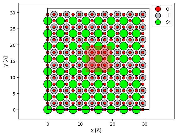
Figure 7:Position and size of the grid scan for a sample of 8x8x24 unitcells of SrTiO3
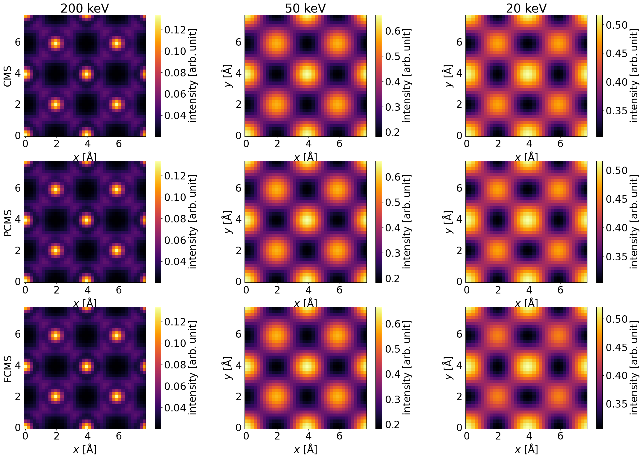
Figure 8:Grid scan with converged probe of 2x2 unitcells SrTiO3
Just looking at these images there does not seem to be any difference across the three multislice implementations. To quantify the difference we will calculate the relative difference for the PCMS and FCMS with the CMS and plot them on the same scale determined by the absolute highest value in all plots.
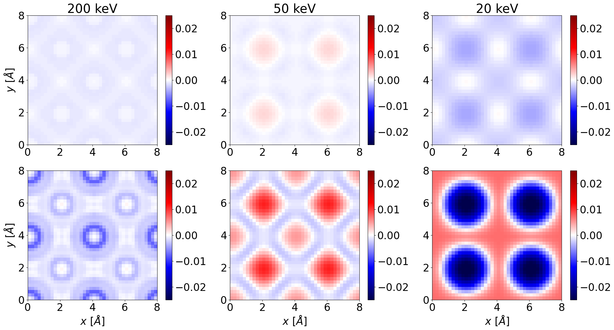
Figure 9:Relative difference plot for PCMS (top row) and FCMS (bottom row) using Figure 8
Here we observe the maximum relative difference increasing for lower energies. Note that, for the 200 kV beam the difference is entirely negative, meaning the new methods predict less electrons scattering on the annular detector. In the other two plots we see a greater dependence on probe position where the PCMS and FCMS predict more scattering on top of the titanium atoms.
Performance
To demonstrate the increased computation time we perform all three methods on a sample of one unit cell of SrTiO3 for various sampling distances. Both the PCMS and FCMS were calculated up to a power of 3 like in previous chapters.
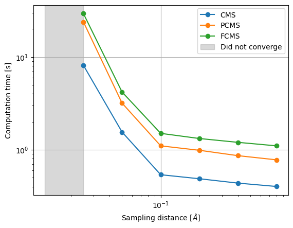
Figure 10:Computation time for one unitcell of SrTiO3 for various sampling distances on log scale